Solving Time-Indepdendent PDEs

Teng-Jui Lin

Content adapted from UW CHEME 375, Chemical Engineering Computer Skills, in Spring 2021.

• Python skills and numerical methods

  • Finite difference method for PDEs

• ChemE applications

  • Time-independent 2D heat transfer

Time-independent 2D heat transfer

Problem Statement. We have a thin metal slab at steady-state, having different temperatures on its four sides. Determine the equilibrium temperature of the slab of points in the interval $[1,3]\times [1,3]$ with equal spacing of 1.

Given boundary conditions $T(0,y)=75{}^{\circ }\mathrm{C},T(4,y)=50{}^{\circ }\mathrm{C},T(x,0)=0{}^{\circ }\mathrm{C},T(x,4)=100{}^{\circ }\mathrm{C}$.

Analytic expression

Solution. We have the heat transport governing equation

$$k{\mathrm{\nabla }}^{2}T+\dot{q}+\mathrm{\Phi }=\rho C_V{\displaystyle \frac{\partial T}{\partial t}}$$

where ${\mathrm{\nabla }}^2=\frac{{\partial }^2}{\partial x^2}+\frac{{\partial }^2}{\partial y^2}+\frac{{\partial }^2}{\partial z^2}$.

Based on the problem statement, we have the assumptions:

• No heat source/generation

  • $\dot{q}=0$

• No fluid or heat movement

  • $\mathrm{\Phi }=0$

• Steady-state system $⟹$ no time dependence

  • $\frac{\partial T}{\partial t}=0$

• Thin metal slab $⟹$ 2D heat transfer (no heat transfer in $z$ direction)

  • $\frac{{\partial }^{2}T}{\partial z^2}=0$

• Constant thermal conductivity $⟹k\ne f(x,y,z,t)$

  • $k$ can be simplified

Therefore, we can simplify the governing equation:

$$\begin{array}{r}\begin{array}{rl}k{\mathrm{\nabla }}^{2}T+\dot{q}+\mathrm{\Phi }& =\rho C_V{\displaystyle \frac{\partial T}{\partial t}}\\ k{\mathrm{\nabla }}^{2}T& =0\\ {\mathrm{\nabla }}^{2}T& =0\\ (\frac{{\partial }^2}{\partial x^2}+\frac{{\partial }^2}{\partial y^2}+\frac{{\partial }^2}{\partial z^2})T& =0\\ \frac{{\partial }^{2}T}{\partial x^2}+\frac{{\partial }^{2}T}{\partial y^2}& =0\end{array}\end{array}$$

Numerical approximations

By central finite difference, we approximate the derivatives by

$${\displaystyle \frac{{\partial }^{2}T}{\partial x^2}}\approx {\displaystyle \frac{T_{i-1,j}-2T_{i,j}+T_{i+1,j}}{\mathrm{\Delta }{x}^2}}$$

$${\displaystyle \frac{{\partial }^{2}T}{\partial y^2}}\approx {\displaystyle \frac{T_{i,j-1}-2T_{i,j}+T_{i,j+1}}{\mathrm{\Delta }{y}^2}}$$

Assume that the spacing in $x$ and $y$ directions are the same $\mathrm{\Delta }x=\mathrm{\Delta }y=1$, we have from the original equation:

$$\begin{array}{r}\begin{array}{rlrl}\frac{{\partial }^{2}T}{\partial x^2}& +& \frac{{\partial }^{2}T}{\partial y^2}& =0\\ {\displaystyle \frac{T_{i-1,j}-2T_{i,j}+T_{i+1,j}}{\mathrm{\Delta }{x}^2}}& +& {\displaystyle \frac{T_{i,j-1}-2T_{i,j}+T_{i,j+1}}{\mathrm{\Delta }{y}^2}}& =0\\ T_{i-1,j}-2T_{i,j}+T_{i+1,j}& +& T_{i,j-1}-2T_{i,j}+T_{i,j+1}& =0\end{array}\end{array}$$

For each point in the slab, we write out the expression from the above equation. We also replace the boundary conditions with numerical values. For example, at point $(i,j)=(1,1)$, we have

$$\begin{array}{r}\begin{array}{rl}{T}_{0,1}-2T_{1,1}+T_{2,1}+T_{1,0}-2T_{1,1}+T_{1,2}& =0\\ T_{0,1}+T_{1,0}-4T_{1,1}+T_{1,2}+T_{2,1}& =0\\ -4T_{1,1}+T_{1,2}+T_{2,1}& =-T_{0,1}-T_{1,0}\\ -4T_{1,1}+T_{1,2}+T_{2,1}& =-75\end{array}\end{array}$$

From PDE to linear algebra

We can repeat the process for all the points. In this case, we have 9 points, therefore 9 equations and 9 unknowns:

$$\begin{array}{r}\begin{array}{ccccccccccc}+4T_{1,1}& -T_{2,1}& & -T_{1,2}& & & & & & =& 75\\ -T_{1,1}& +4T_{2,1}& -T_{3,1}& & -T_{2,2}& & & & & =& 0\\ & -T_{2,1}& +4T_{3,1}& & & -T_{3,2}& & & & =& 50\\ -T_{1,1}& & & +4T_{1,2}& -T_{2,2}& & -T_{1,3}& & & =& 75\\ & -T_{2,1}& & -T_{1,2}& +4T_{2,2}& -T_{3,2}& & -T_{2,3}& & =& 0\\ & & -T_{3,1}& & -T_{2,2}& +4T_{3,2}& & & -T_{3,3}& =& 50\\ & & & -T_{1,2}& & & +4T_{1,3}& -T_{2,3}& & =& 175\\ & & & & -T_{2,2}& & -T_{1,3}& +4T_{2,3}& -T_{3,3}& =& 100\\ & & & & & -T_{3,2}& & -T_{2,3}& +4T_{3,3}& =& 150\end{array}\end{array}$$

so we have the system $\mathbf{A}\mathbf{x}=\mathbf{b}$, where

$$\begin{array}{r}\mathbf{A}=\left[\begin{array}{ccccccccc}+4& -1& & -1& & & & & \\ -1& +4& -1& & -1& & & & \\ & -1& +4& & & -1& & & \\ -1& & & +4& -1& & -1& & \\ & -1& & -1& +4& -1& & -1& \\ & & -1& & -1& +4& & & -1\\ & & & -1& & & +4& -1& \\ & & & & -1& & -1& +4& -1\\ & & & & & -1& & -1& +4\end{array}\right],\mathbf{x}=\left[\begin{array}{c}{T}_{1,1}\\ T_{2,1}\\ T_{3,1}\\ T_{1,2}\\ T_{2,2}\\ T_{3,2}\\ T_{1,3}\\ T_{2,3}\\ T_{3,3}\end{array}\right],\mathbf{b}=\left[\begin{array}{c}75\\ 0\\ 50\\ 75\\ 0\\ 50\\ 175\\ 100\\ 150\end{array}\right]\end{array}$$

We can then solve the system of linear equations.

Implementation

In this approach, we use numpy.linalg.solve() to solve the linear system obtained from simplifying the PDE.

import numpy as np
import matplotlib.pyplot as plt

# create the (sparse) matrix
A_size = 9
A = np.zeros((A_size, A_size))
for i in range(A_size):
    A[i, i] = 4

band_num = 4-1
for i in range(A_size-band_num):
    A[3+i, i] = -1
for i in range(A_size-band_num):
    A[i, 3+i] = -1

band_num = 2-1
for i in range(A_size-band_num):
    A[band_num+i, i] = -1
for i in range(A_size-band_num):
    A[i, band_num+i] = -1
    
for i in range(2, A_size-band_num, 3):
    A[band_num+i, i] = 0
for i in range(2, A_size-band_num, 3):
    A[i, band_num+i] = 0
A

array([[ 4., -1.,  0., -1.,  0.,  0.,  0.,  0.,  0.],
       [-1.,  4., -1.,  0., -1.,  0.,  0.,  0.,  0.],
       [ 0., -1.,  4.,  0.,  0., -1.,  0.,  0.,  0.],
       [-1.,  0.,  0.,  4., -1.,  0., -1.,  0.,  0.],
       [ 0., -1.,  0., -1.,  4., -1.,  0., -1.,  0.],
       [ 0.,  0., -1.,  0., -1.,  4.,  0.,  0., -1.],
       [ 0.,  0.,  0., -1.,  0.,  0.,  4., -1.,  0.],
       [ 0.,  0.,  0.,  0., -1.,  0., -1.,  4., -1.],
       [ 0.,  0.,  0.,  0.,  0., -1.,  0., -1.,  4.]])

b = np.array([75, 0, 50, 75, 0, 50, 175, 100, 150])

temperatures = np.linalg.solve(A, b)
temperatures

array([42.85714286, 33.25892857, 33.92857143, 63.16964286, 56.25      ,
       52.45535714, 78.57142857, 76.11607143, 69.64285714])

row = 3
col = 3
T_profile = temperatures.reshape(row, col)

for i in np.arange(6, -1, -3):
    print('{:.2f} | {:.2f} | {:.2f}'.format(*temperatures[i:i+3]))

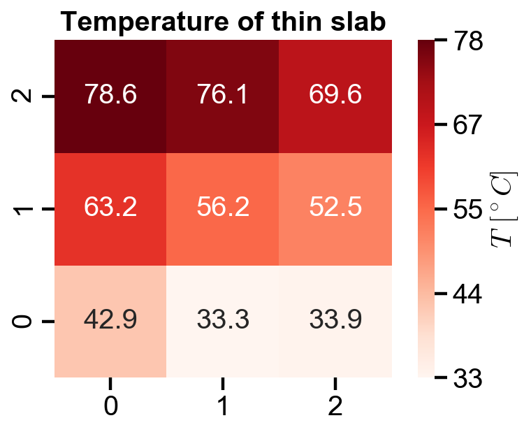
78.57 | 76.12 | 69.64
63.17 | 56.25 | 52.46
42.86 | 33.26 | 33.93

Plotting annotated heatmap

# plot settings
%config InlineBackend.figure_format = 'retina'
%matplotlib inline

plt.rcParams.update({
    'font.family': 'Arial',  # Times New Roman, Calibri
    'font.weight': 'normal',
    'mathtext.fontset': 'cm',
    'font.size': 18,
    
    'lines.linewidth': 2,
    
    'axes.linewidth': 2,
    'axes.spines.top': False,
    'axes.spines.right': False,
    'axes.titleweight': 'bold',
    'axes.titlesize': 18,
    'axes.labelweight': 'bold',
    
    'xtick.major.size': 8,
    'xtick.major.width': 2,
    'ytick.major.size': 8,
    'ytick.major.width': 2,
    
    'figure.dpi': 80,
    
    'legend.framealpha': 1, 
    'legend.edgecolor': 'black',
    'legend.fancybox': False,
    'legend.fontsize': 14
})

import seaborn as sns
T_heatmap = sns.heatmap(T_profile, square=True, cbar=True,
                        annot=True, fmt=".1f", cmap='Reds',
                        cbar_kws={'label': '$T \ [^\circ C]$', 
                                  'format': '%i', 
                                  'ticks': np.linspace(temperatures.min(), temperatures.max(), 5)})
T_heatmap.set_title('Temperature of thin slab')
T_heatmap.invert_yaxis()